

Energy Performance of Buildings as a User Driven Process
Abstract
Energy performance calculations of buildings due to national and European standards show a very weak correlation between the real (measured) energy consumption and the in this way calculated (see energy certificates) energy demand. In several research works the squared correlation coefficient had been computed to roundabout r2 ≈ 0.2 only. Some reasons for these discrepancies can be related to the scattering weather conditions and seen as caused by the real indoor temperature according to building users comfort expectations. Result of such calculations will be not a deterministic value but the frequency distribution of the building energy demand.
1. Comparing calculated energy performance with metered energy consumption
During the last decades there has been performed several Europe-wide studies correlating the metered energy consumption with the calculated energy performance (energy demand stated nowadays by building energy certificates).
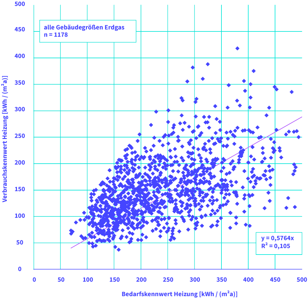
Figure 1: Correlating metered (vertical axis) energy consumption with calculated (horizontal axis) energy performance of gas heated residential buildings (see: Jens Knissel, Roland Alles, Rolf Born, Tobias Loga, Konny Müller, Verena Stercz: Entwicklung eines vereinfachten Verfahrens zur Ermittlung gebäudespezifischer Primärenergiekennwerte, geeignet als Bewertungsmerkmal im Mietspiegel, research report, July 2006).
An example for such an investigation is given by fig. 1. Not only from fig. 1 but also from all of these research works can be drawn the same conclusion:
- The squared coefficient of correlation is only in the range of 0.2, so that the real (metered) energy consumption is dominated to round about 80 % by other influences as the building performance.
- Besides the scattering of the values, is the metered energy consumption missing systematically and in average overestimating the calculated energy demand.
- Nevertheless, based on this energy performance with a high risk for false conclusions are:
- Building energy certificates implemented as an energy steering element of the real estate market.
- Investment and financing decisions of building owners willing to do energetically rehabilitation but also of banks offering special loans for their financing (supported sometimes by tax money).
- Climate protection targets.
- Policy tools on national and European level (energy saving laws as well as EPBD of the EU are using energy calculation models without minding the gap of its results to the real energy consumption).
2. Calculation of the energy performance of residential buildings
The energy performance of residential buildings can be calculated in an easy way if it is based on the following basic assumptions (s. Tab. 1):

Table 1. Basic assumptions and idealisations of the building heating energy calculation model.
Calculations will be done here only for the above mentioned residential building. According to the assumptions of tab.1 the total heat demand of the building can be calculated to 124 kWh/(m2∙year).
3. Probabilistic energy performance calculation of residential buildings
3.1 Relevance
For example the city council of Zurich (see: TEC 21, no. 7, 2012, page 28ff) had researched that building users can activate and realize by their behaviour an energy saving potential in the range of 20 to 30 percentage (heating and domestic hot water) without investing in technical improvements of their buildings and without “sitting in the dark and freeze” (by ongoing indoor comfort).
In 2007 the Bremer Energy Institute had have investigated 676 single family houses concerning their energy consumption in the period from 1997 to 2006. For 56 single family houses of them had been noticed an energy consumption reduction of more than 35 %. Round about one-fourth of these 56 households had reached this without any investment in building renovation measures.
Both examples give an impression that it is by ignoring the user behaviour not possible to calculate a sound and realistic value of the building heat consumption.
Such saving aspects are one reason to switch the focus concerning building energy demand from building construction to building user. The scattering of the energy consumption noticed and occurring (see fig. 1) in buildings with the same conditions (identical energy performance) obviously (not surprisingly) related in first line to the following two effects:
- Scattering of the weather conditions and
- Scattering of the indoor temperature due to the behaviour and comfort wishes of the building user.
3.2. Weather conditions
Exemplarily the following analysis and calculations are performed for a building location in Potsdam. The cycle of the average day temperature according to DIN 4710 is given by fig. 2.
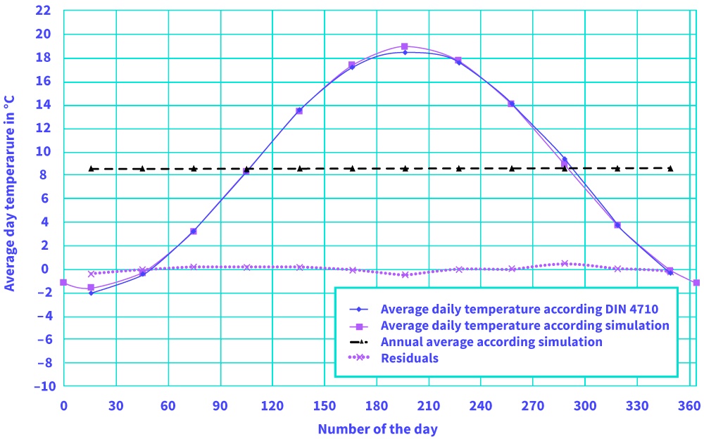
Figure 2: Annual cycle of the average daily outdoor temperature in Potsdam (DIN 4710 and own approximation)
This cycle can be approximated as an unsymmetrical cosine-wave. This approximation is used to calculate the heating degree days in dependency of the indoor temperature chosen by the building user. Assumed is therefore a heating limited temperature which is 3 K lower as this indoor temperature. The in this way calculated heating degree days are given with fig. 3.
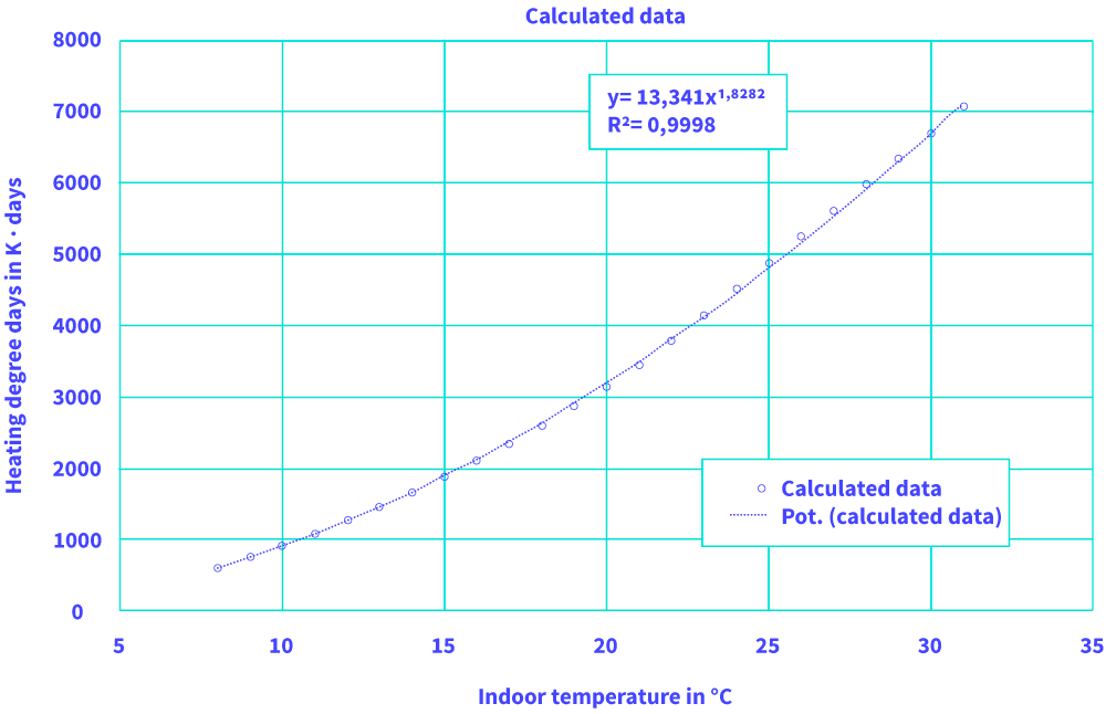
Figure 3: Calculated heating degree days according to Potsdam weather conditions given by fig. 2 and it’s approximation by a power function (own calculation)
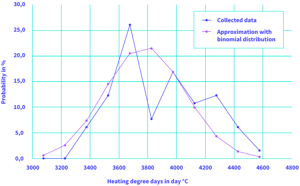
Figure 4: Frequency distribution of heating degree days of Potsdam and its approximation by binomial distribution (data from www.modernus.de/heizgradtage/potsdam, called at 08.09.2015)
The scattering of this average weather conditions can be described by the frequency distribution of published heating degree days (see fig. 4).
3.3. Indoor temperature conditions in residential buildings
The Technical University of Dresden had have measured indoor temperatures in residential buildings from 2005 to 2008. In these years they had done 3.7 million measurements between November and April only (published in: EnEV aktuell, no. 1, 2010). The frequency distributions of these measurements are given by fig. 5. They can be approximated by a normal distribution with average of 18.3 °C and a standard deviation of 3.5 °C.
Based on these data (see fig. 2 – 5) and the same simple calculation model of the building heat demand (see chapter 2) a Monte-Carlo-Simulation is executed. More details of this calculation can’t be explained here.
4. Calculation of the probability distribution of the heat demand
The result of this simulation is given in figure. 6. The average heat demand according to this simulation is 93 kWh/(m2 ∙ year). As expected to common research results (remember fig. 1): This is related to the deterministic value of 124 kWh/(m2 ∙ year) (see chapter 2) 25 % lower. Conclusion: When using realistic indoor temperature conditions instead of a fixed 20 °C value, than energy demand calculations much closer to metered energy consumption values.

Figure 5: Metered indoor temperatures (see: EnEV aktuell, no. 1, 2010)
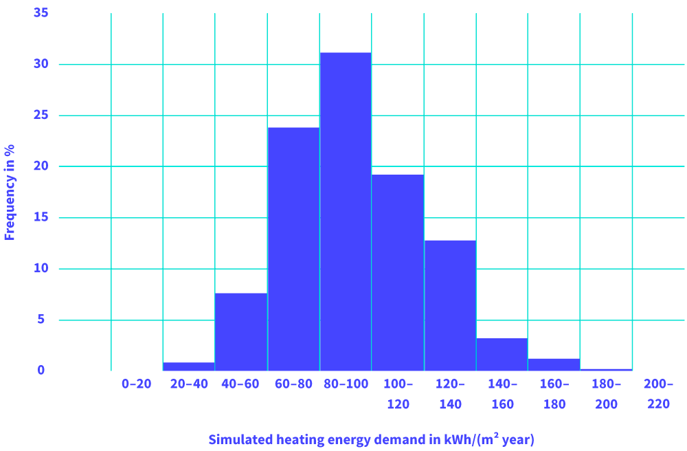
Figure 6: Probability distribution of heat energy demand (own calculation)
- Back